
[aug 26] grokfast paper notes
- Gradient updates can be decomposed into fast-varying and slow-varying components.
- fast varying components contribute to overfitting and slow-varying ones to generalization.
- They accelerate generalization under grokking by amplifying the low-frequency part of the optimizer’s gradient using LPF.
- Grokking is a state transition phenomenon.
With \(g(t) = \frac{\partial l(t)}{\partial \theta(t)}\), we have this simple discrete optimizer abstraction:
\[\theta (t+1) = \theta(t) + u(g(t), t) = \theta (0) + \sum^T_{\tau = 0}u(g(\tau), \tau)\]Since optimization a collection of discrete random signals \(u(t)\), it’s dual representation \(U(w)\) in the frequency domain is:
\[U(w) = \mathcal{F}\{u(t)\} = \sum^T_{t=0} u(t)e^{-iwt}\]Since they assume grokking is linked to slow varying compononents of \(u(t)\), it will be related to low frequency part of \(U(w)\). \(U(w)\) can be represented by \(G(w) = \sum^T_{t=0}g(t)e^{-iwt}\) since optimizer are first order with \(g(t)\) linearly correlated with \(u(t)\).
Low Pass Filter - Grokfast MA
\(\hat{g}(t)\) convolved gradient \(g(t)\) by a univariate time-invarient LPF \(h(t)\) :
\[\hat{g}(t) = g(t) + h(t) * g(t) \text{, and in frequency domain : } \hat{G}(w) = G(w) + H(w)G(w) = (1+H(w))G(w)\]so
\[\hat{u}(t) = u(\hat{g}(t), t) = u( g(t) + h(t) * g(t), t)\]The goal is to design a filter \(h(t)\) with low pass proprieties in \(H(w)\): window moving average (MA) over fixed size window of width \(w\):
\[h(t) = \begin{cases} \lambda / w &\quad\text{if } 0 \le t \lt w\\ 0 &\quad\text{otherwise} \end{cases}\]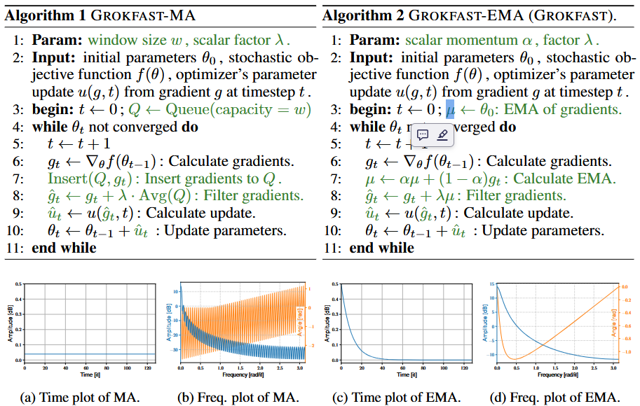
One major flaw is the memory scaling: you need \(w\) times more memory than originaly needed + non linear training time scaling. So non applicable to actual big models.
Exponential Moving Average LPF
New LPF with smaller memory footprint (size of the model params)
\[h(t) = \lambda(1-\alpha)\sum^t_{\tau = 0}\alpha^{\tau}\delta(t-\tau) = \lambda\alpha^t(1-\alpha)\]with \(\delta(t)\) the discrete unit impule at the origin.
We can then express the convolution \(\mu_t = \sum_{\tau = 0}^t h(\tau)g_{t-\tau}\) as a recursive algorithm:
\[\begin{align} \mu_t &= \sum_{\tau = 0}^t h(\tau)g_{t-\tau} \\ &= \sum_{\tau = 0}^t \alpha^{\tau}(1-\alpha)g_{t-\tau} \\ &= (1-\alpha)g_t + \sum_{\tau = 1}^t \alpha^{\tau}(1-\alpha)g_{t-\tau} \\ &= (1-\alpha)g_t + \alpha\sum_{\tau = 1}^t \alpha^{\tau-1}(1-\alpha)g_{t-\tau} \\ &= (1-\alpha)g_t + \alpha\sum_{\sigma = 0}^{t-1} \alpha^{\sigma}(1-\alpha)g_{(t-1) - \sigma} \\ &= (1-\alpha)g_t + \alpha \mu_{t-1} \end{align}\]Discussion
- Removing fast gradient result in a delayed and unstable generalization
- State transition can be exploited for faster generalization under grokking (apply MA only after overfitting)
- Following Omnigrok[1], weight decay accelerate generalization under grokking.
Trajectories
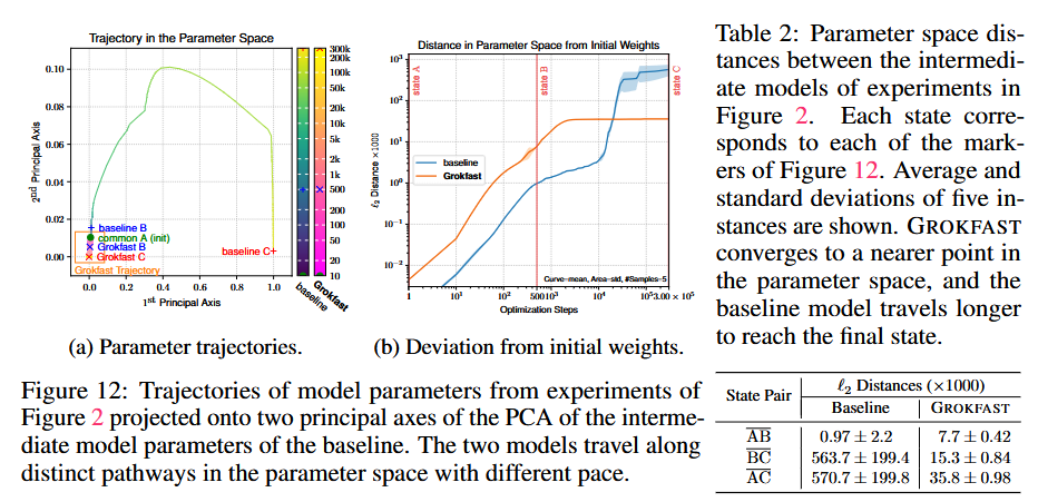
Theses observations support the interpretation that grokking is a state transition phenomenon.
References
[1] Kumar et al. Grokking as the Transition from Lazy to Rich Training Dynamics. 2023 cs.LG