Spectral Entropy Dynamics in Deep Linear Networks

• Intuition
• Computing \(\dot{p}_{\alpha}\)
• 2. Phase de généralisation
• 3. Mémorisation

Intuition

Can we track overparametrized linear network learning only with a single scalar ?

Saxe tell us that in a DLN, learning is sequential and hierarchical : from important low frequeny signal to high frequency signal. He also give us :

\[a_{\alpha}(t)=\frac{s_{\alpha}e^{2_{\alpha}t/{\tau}}}{e^{2s_{\alpha}t/{\tau}} - 1 + s_{\alpha}/a_{\alpha}^0}\]

It allowed to derive:

• which mode is learning first
• when the network start to learn the noise
• if this sequential and hierarchical properties allow us to approximate an optimal stopping point for learning ?

So the main tool will be spectral entropy: \(H(t) = - \sum_\alpha p_\alpha \log p_\alpha\)

with :

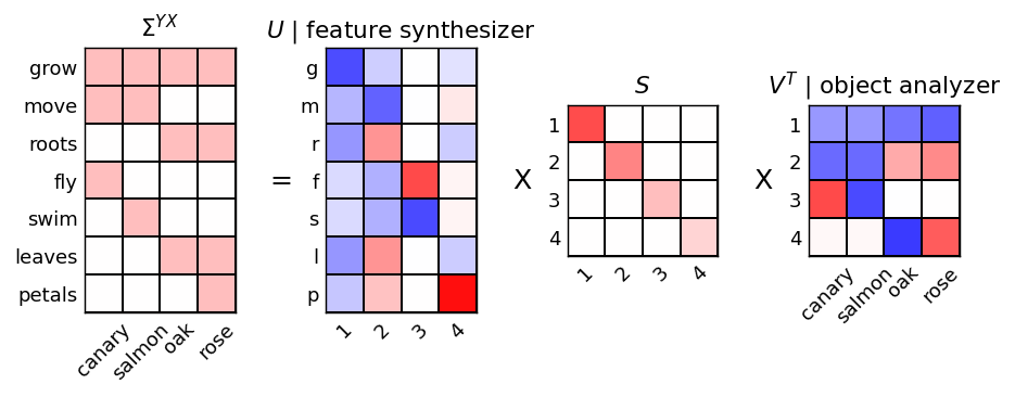
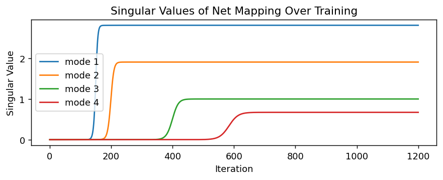
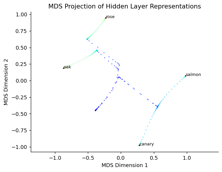
\[p_\alpha = \frac{a_\alpha^2}{\sum_\beta a_\beta^2}\]

We start with the same setup as saxe leading to this covariance, mds projection, spectral dynamics and entropy:

And by plotting the entropy we end up with this:

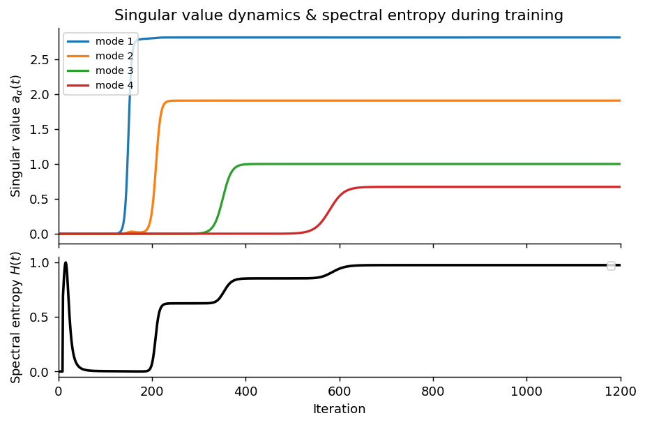
As we know:

• low entropy means that only a few modes dominates
• high entropy : energie is spread accros the modes

Some intuitions:

• If signal to noise ratio is higher, or \(dim -> \infty\), maybe ye’ll loose the “cascade” effect of the entropy ?

Résultat principal : covariance identity

En dérivant :

\[\begin{align} H(t) = -\sum_{\alpha}p_{\alpha}(t)log(p_{\alpha}(t)) \end{align}\]

so

\[\begin{align} \dot{H}(t) &= \sum_{\alpha} d/{dt} (p_{\alpha}log(p_{\alpha}))\\ d/{dt}(p.log(p)) &= \dot{p}log(p) + p\dot{p}/p \\ &= \dot{p}(log(p) + 1)\\ \dot{H} &= \sum_{\alpha} \dot{p_{\alpha}}(log(p_{\alpha}) + 1)\\ &= \sum_{\alpha} \dot{p_{\alpha}}log(p_{\alpha}) \text{ because } \sum_{\alpha} p_{\alpha} = 1. \end{align}\]

Computing \(\dot{p}_{\alpha}\)

\[p_{\alpha} = \frac{a_{\alpha}^2}{S}, S = \sum_{\beta}a_{\beta}^2\] \[\begin{align} \dot{p}_{\alpha} &= \frac{2a_{\alpha}\dot{a_{alpha}}S - a^2_{\alpha}\dot{S}}{S^2} \\ &= \frac{2a_{\alpha}\dot{a_{\alpha}}S - 2a^2_{\alpha}\sum_{\beta}a_{\beta}\dot{a}_{\beta}}{S^2} \\ &=\frac{2a^2_{\alpha}}{S}(\frac{\dot{a}_{\alpha}}{a_\alpha} - \frac{\sum_{\beta}a_{\beta}\dot{a}_{\beta}}{S}) \\ \sum_{\beta}\frac{a^2_{\beta}}{S}\frac{\dot{a}_{\beta}}{a_{\beta}} = \sum_{\beta}p_{\beta}g_{\beta} \\ &=2p_{\alpha}(g_{\alpha} - E_p[g])\\ \dot{H}(t)&=-\sum_{\alpha}2p_{\alpha}(g_{\alpha} - E_p[g])log(p_{\alpha})\\ &=-2\sum p_{\alpha}g_{\alpha}log(p_{\alpha}) + 2E_p[g]\sum p_{\alpha} log(p_{\alpha})\\ &=-2(E_p[g.log(p)] - E_p[g]E_p[log(p)])\\ &=-2Cov(g_{\alpha}, log(p_{\alpha})) \end{align}\]

then \(g_{\alpha} = \frac{\dot{a}_{\alpha}}{a_{\alpha}}\) is the relative rate of change. And \(log(p)\) is nice because it emphasize which mode is small and which one is huge, so \(Cov(g_{\alpha}, log(p_{\alpha}))\) tells us if faster learned modes are small or big: we know the answer from Saxe, but good to know the insight of \(H\).

Cette formule explique les trois phases d’apprentissage.

Au début :

• les modes importants grandissent vite,
• les petits modes sont encore absents.

Donc :

• gros \(g_\alpha\),
• petits \(p_\alpha\).

Cela réduit l’entropie :

\[\dot H < 0\]

Le réseau concentre son énergie sur quelques directions dominantes.

---

2. Phase de généralisation

À un certain moment :

• les grands modes ont saturé,
• les petits modes n’ont pas encore démarré.

Le système atteint un équilibre :

\[\dot H \approx 0\]

Le réseau représente correctement la structure principale des données.

---

3. Mémorisation

Ensuite :

• les modes bruit commencent à croître,
• ils ont encore une faible énergie,
• mais leur taux de croissance est grand.

Cela redistribue l’énergie sur beaucoup de directions :

\[\dot H > 0\]

Le réseau commence à apprendre des détails fins et du bruit.

---

Fenêtre de stopping

On définit :

• \(t^*\) : minimum de l’entropie,

• \(t^{**}\) : début de la phase de mémorisation.

Le résultat important :

\[t^* \le t_{\mathrm{opt}} \le t^{**}\]

où :

\[t_{\mathrm{opt}}\]

est le meilleur temps d’arrêt pour la généralisation.

---

Intuition

Avant \(t^*\) :

• les modes importants ne sont pas encore appris.

Après \(t^{**}\) :

• le bruit commence à être appris.

Donc la meilleure généralisation doit se situer entre les deux.

Cela donne une version dynamique du early stopping :

arrêter avant que les modes bruit deviennent dominants.

---